Don’t count the days, make the days count.
Mohammed Ali
LifeLogging is nice — you leave lots of data which tells you more about yourself than you usually find out by remembering what you did, and when. Especially when it comes to daily activities and habits. However, data does not tell you much unless you find a good way to visualize the data.
I’m really becoming a fan of R, especially with tidyverse. Adding lubridate to deal with dates doesn’t hurt either.
And it’s fun what you can find out. For example, suppose you had access to data on your work time, for example, because you punch in and out every day (and for your lunch break). Even without being mandated, you could do so easily with apps like DueTime (as long as you remember to swipe the bar at the bottom to the left to see the export options, seriously, DueTime, what the hell?!?!). Even if you did not log work outside of the office, or at weekends, it would provide lots of interesting information.
So, what could this data tell you? Let’s take this sample data:
Cumulative Overtime
For example, you can compare the hours you worked over the course of your contact (blue) and the hours you should have worked (red):
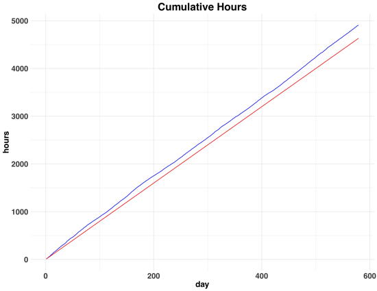
So, there is a gap and it’s widening over time. It’s not that there’s a little overtime here, it’s overtime that adds up and grows larger and larger. The disadvantage with this graph — it’s kinda hard to see what the overtime has accumulated to be — about 273 hours, or 11 full days, or 34 workdays.
Hours Worked per Day
How do these hours translate to a typical workday? A simple histogram shows the hours worked per day.
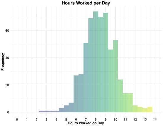
More or less normally distributed, with a mean of 8.47 hours (without lunch), SD = 1.65, and a range of 11.52 (2.28 to 13.8). Some very short days, but some rather long ones).
Beginning and End of the Workday
Having both the start (orange) and end times (blue) of each workday allows you to plot both in a nice histogram.
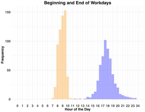
The difference in variance is not surprising, considering most jobs have times when you should be at work. The stop time standard deviation (SD = 1.5) is much larger than the start time variance (SD = 0.79).
So, yeah, interesting to look into these sample data. You usually don’t see data aggregated this way. Yeah, you might have an idea, but seeing the numbers …
But yeah, even playing around with some sample data — question still is, what kind of conclusions could you draw? And also, if time outside of the office wasn’t tracked in this case, how high would the full work hours number be? And if this much time is spend on one thing, is it really worth it?
And yeah, R is pretty cool here.